
A Quick Look at Neural Ordinary Differential Equations
Published:
Exploring the basic ideas behind Neural ODEs
We can describe many natural processes via differential equations: the motion of objects, population dynamics, and options prices. As a physics student, I’ve had my fair share of playing with differential equations in math models. The goal of creating models is to approximate nature, allowing us to make predictions and extract insights from (often complex) underlying processes. This goal closely aligns with the broader aim of machine learning: to develop algorithms that can learn patterns and make predictions from data.
In (supervised) machine learning, we’re given a data set \(\mathcal{D}\) with \(n\) data points:
\[\mathcal{D} = \{ (x_1, y_1), (x_2, y_2), \ldots, (x_n, y_n)\}\]Goal: given an unseen data point \(x'\), how do we build a model to predict the corresponding \(y'\) ?
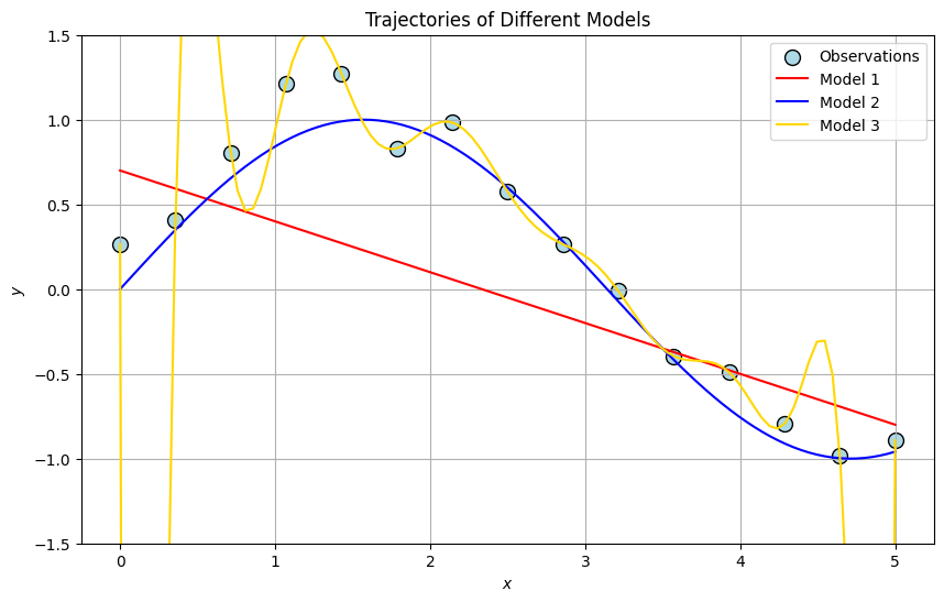
The usual approach is to approximate nature’s data-generating function \(f\) with a machine learning model (say, a neural network) \(\widehat{f}\). Assuming we’re sophisticated enough to create a good approximation, then we expect for some unseen data point \(x'\),
\[f(x') \approx \widehat{f}(x')\]To make good predictions requires building and training sufficiently robust models that generalizes well to new data.
Training Neural Networks
Let’s recall what the typical training loop of a neural network looks like:
Forward pass: make predictions with the neural network
\[\text{Predictions} = \text{NN}(\text{Input Data})\]Remember, neural networks are functions. That is, a neural network simply takes in a number/vector and spits out a number/vector as a prediction.
Compute loss: calculate neural network error
Loss quantifies the error between model predictions and true/expected outputs. We have numerous ways of calculating loss such as mean squared error (MSE) and mean absolute error (MAE):
\[\text{MSE} = \frac{1}{n} \sum_{i=1}^{n} (y_i - \hat{y}_i)^2\] \[\text{MAE} = \frac{1}{n} \sum_{i=1}^{n} |y_i - \hat{y}_i|\]where \(y_i\) is the “true value”, \(\hat{y}_i\) is the model’s predicted value, and \(n\) is the number of data points. The choice of loss function depends on the given problem (what types of errors should be penalized the most, and by how much?). Regardless of loss function, we want to adjust neural network parameters to minimize loss.
Machine learning now becomes an optimization problem: how do we tune our model’s parameters to obtain the smallest loss?
Backward pass: calculate gradients with respect to the loss
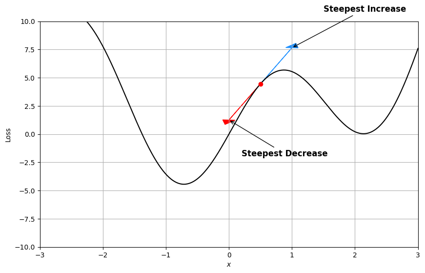
Recall that the gradient of a function tells us the direction of steepest increase. In the context of optimization, we’re interested in the steepest decrease, which happens to be the opposite direction. We can take the derivative (gradient) of the loss function with respect to the model parameters to decrease our loss
Optimizer step: update model parameters
After obtaining the gradient, we can move in the direction (update parameters) that most decreases our loss. The optimizer calculates how much and in which direction to adjust model parameters.
The Big Picture of NeuralODEs
Neural Ordinary Differential Equations (NeuralODEs) instead approximate something slightly different: rather than directly predicting outputs from inputs, they model the derivative of the data-generating function.
Suppose we have a set of \(n\) observations \(\{ (t_0, \mathbf{z_0}), (t_1, \mathbf{z_1}) \ldots, (t_n, \mathbf{z_n})\}\) governed by the system of ordinary differential equations:
\[\frac{d\mathbf{z}}{dt} = f(\mathbf{z}(t), t)\]The core idea behind NeuralODEs is to replace \(f\) with a neural network \(NN\) using our observations as training data:
\[\frac{d\mathbf{z}}{dt} = NN(\mathbf{z}(t), t)\]Since ODEs appear in many fields, we have numerous methods to approximate their solutions. Modeling data as a differential equation allows us to make continuous-time predictions and can provide a better understanding of the underlying mechanisms.
Connecting ResNets to Euler’s Method
To understand the motivation behind NeuralODEs, we have to revisit Euler’s method.
Recall that we can approximate the derivative (gradient) of some function \(z(t)\) with
\[\frac{dz}{dt} \approx \frac{z(t+\Delta t) - z(t)}{\Delta t}\]for some small value \(\Delta t\), which we will call the step-size. A simple rearrangement yields:
\[z(t + \Delta t) \approx z(t) + \Delta t \frac{dz}{dt}\]We use the expression above to approximate points of \(z(t)\), denoted as \(z_i\), assuming we have some starting point \(z_0\) with the following recursive formula:
\[z_{n+1} = z_n + \Delta t \frac{dz}{dt}, \quad n = 0, 1, 2, \ldots\]The gradient \(\frac{dz}{dt}\) tells us in which direction to move, and \(\Delta t\) tells us by how much (smaller \(\Delta t\) gives better approximations at the cost of more computation since we take many more small steps to reach the same end point).
How does this relate to machine learning? Well, let’s take another look at neural networks:
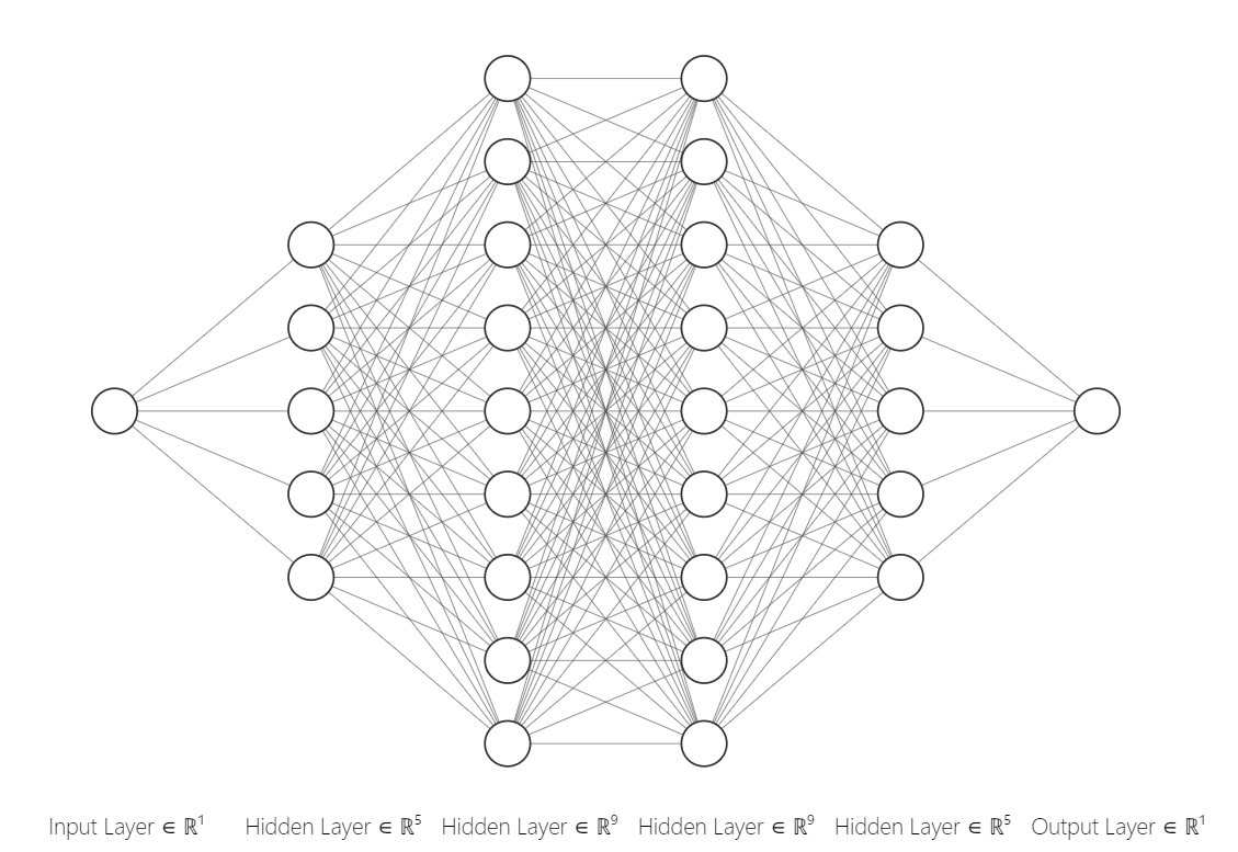
Source
A neural network with hidden layers transforms inputs into hidden states as data passes through the network. Each hidden layer of the neural network is a function itself (a neural network is a composition of many functions).
Let \(f\) be the function that maps a hidden state \(h_i\) to the subsequent hidden state \(h_{i+1}\). As inputs, \(f\) takes in outputs from the previous hidden layer \(h_t\) and parameters (i.e weights and biases) \(\theta_t\). We can write a recursive formula for how inputs propogate through the neural network:
\[h_{t+1} = f(h_t, \theta_t)\]Now, consider a common neural network architecture called Residual Neural Networks (ResNets). ResNets introduce shortcut connections that allow information to bypass intermediate layers, meaning the output of a hidden layer can include contributions from multiple preceding layers. ResNets were initially developed to improve gradient stability while training neural networks. In the case where a layer takes in outputs from the previous two layers, we modify the above formula slightly:
\[h_{t+1} = h_t + f(h_t, \theta_t)\]Hmm… this looks an awful lot like a recursive formula from Euler’s method. What happens in the limit of more layers and smaller steps (the step size above is \(1\))?
\[\frac{h_{t+1} - h_t}{1} = f(h_t, \theta_t) \to \frac{dh(t)}{dt} = f(h(t), t, \theta)\]What does this mean? We can interpret a ResNet as an Euler’s method approximation to a differential equation! Euler’s method is one of the simplest ways to solve a differential equation. Can we come up with better architecture than ResNets in the same way that there are better numerical methods than Euler’s? Let’s rewrite the differential equation in terms of an integral equation (using \(t'\) as a dummy variable of integration):
\[h_{t+1} = h_t + \int_{t}^{t+1} f(h(t'), t', \theta) dt'\]Remember, the above equation is an exact solution to the hidden states differential equation. We approximate \(h_{t+1}\) using a numerical integration scheme of our choice.
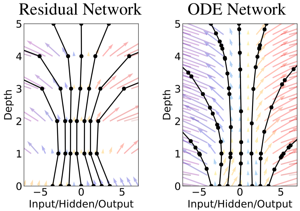
We can see that ODE Networks “smooth out” the hidden states. The key takeaway is to understand that NeuralODEs consist of 2 main components:
- The neural network as the underlying differential equation \(\frac{dz}{dt} = NN(z(t), t)\)
- The numerical ODE solver, which acts as a continuous-depth, improved version of the ResNet architecture.
Training NeuralODEs
But how does one train a NeuralODE?
Forward pass: Solve the differential equation
Given an inital condition \(z(t_0)\), use a numerical solver \(\text{ODESolve}\) to solve the differential equation \(\frac{dz}{dt} = f_{\theta}(z(t), t)\).
Here \(f\) is the neural network (or whatever you’re using) with parameters \(\theta\).
\[z(t) = \text{ODESolve} \left( \frac{dz}{dt} = f_{\theta}(z(t), t), z(t_0)\right)\]We can choose \(\text{ODESolve}\) to be anything we want (Euler’s method, RK4, etc.), which allows us to balance speed and accuracy to our liking.
Compute loss: calculate neural network error
Once we have the trajectory \(z(t)\), we calculate the error (your metric of choice) between the predictions \(z(t_i)\) and the data \(y_i\).
\[\text{Loss} = \frac{1}{n} \sum_{i=1}^{n} \text{loss}(z(t_i), y_i)\]Backward pass: calculate gradients with respect to the loss
Calculating NeuralODE gradients is much different than for standard neural nets. To update \(\theta\), we need the gradient of the loss with respect to the parameters of \(f_\theta\). The authors in the original paper used an adjoint method. I won’t go into the full details in this post (something to do for the future), but it’s an extremely clever method for propogating loss continuously.
In traditional Neural Networks, we can use the chain rule to calculate the gradients with respect to parameter \(\theta_i\):
\[\frac{\partial \mathcal{L}}{\partial \theta_i} = \frac{\partial \mathcal{L}}{\partial y_n} \frac{\partial y_n}{\partial y_{n-1}} \cdots \frac{\partial y_2}{\partial y_1} \frac{\partial y_1}{\partial \theta_i}\]In NeuralODEs, we use an instantaneous analog of the chain rule. The paper uses an adjoint state term \(a(t)\) to arrive at the equation:
\[\frac{\partial L}{\partial \theta} = \int_{t_1}^{t_0}a(t)^T \frac{\partial f(z(t), t, \theta)}{\partial \theta} dt\]Intuitively, the above equation adds up the influence of each time step (scaled by \(a(t)\)) multiplied by the gradient of the output, giving us the “overall” gradient.
Optimizer step: update model parameters
Once we compute the gradients, we can use our optimizer of choice (SGD, Adam, etc) to update the parameters \(\theta\).
Pros and Cons of NeuralODEs
Why would we want to do this in the first place? Well, there are a few advantages:
Efficiency: In some cases, NeuralODEs use less memory and fewer parameters to achieve similar results to architectures such as ResNet.
Choose our tradeoffs: Utilizing NeuralODEs depends on our ODE solver which grants us more flexibility to trade-off between speed and precision
Irregular time series: Fitting time series models especially with irregularly sampled data is difficult. By design, NeuralODEs can handle this much better.
I plan to continue posting about some examples of NeuralODEs in the future.